
Block
Deconvolution
- What it does
- It sharpens the stack, using the shape of the stars measured on the stack itself.
- What it shows
- Tighter stars and finer detail; Inspect shows the image before and after, with the median star width before and after.
- What can be set
- Iterations sets how much it sharpens and Regularization holds back noise and rings; the defaults suit most images.
The Deconvolution block sharpens the stack and its two half-stacks with the shape of the stars measured on the stack itself, zone by zone and colour by colour. The classic method is a Richardson-Lucy iteration that keeps the clipped cores of saturated stars from ringing into the image. A second method, a neural network, is in beta. The block is optional, works on linear data and sits before Denoise.
- Stacking
- Astrometry
- Gradient
- Deconvolution
- Denoise
- Color
1Before and after on a real image
The comparison below uses one project of the Rosette Nebula: 436 exposures of 15 s with a Sony A7S at ISO 4000, on a 130/900 Newtonian. The two images come from the same project, without the Deconvolution block and with it in its method Neural network, in beta. The block sits after Gradient and before Denoise. Everything else is identical, and both are shown with the same stretch; the sky’s level is unchanged. The crops are at 100 %: one image pixel is one screen pixel. The deconvolution took 2.9 min on an RTX 4060 Ti graphics card. Drag the divider, or focus it and use the arrow keys.
| Zone | Box in the stack (x, y) | Star width (median, px) | Stars detected |
|---|---|---|---|
| 1 Cluster on the nebula | 1540–2240, 1120–1820 | – | 729 → 1056 |
| 2 Bright nebula, dark globules | 1550–2250, 520–1220 | – | 555 → 772 |
| 3 Faint arc | 1936–2636, 241–941 | 4.95 → 4.53 (−8 %) | 395 → 530 |
| 4 Star field | 2750–3450, 1070–1770 | 4.84 → 4.19 (−13 %) | 279 → 382 (+37 %) |
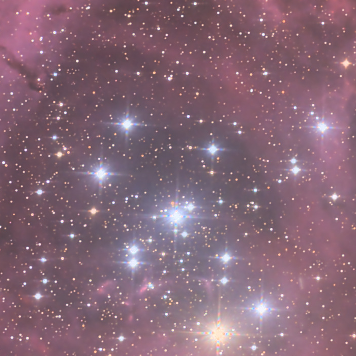 After
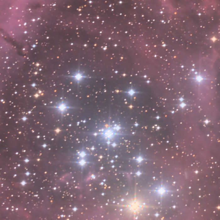 Before
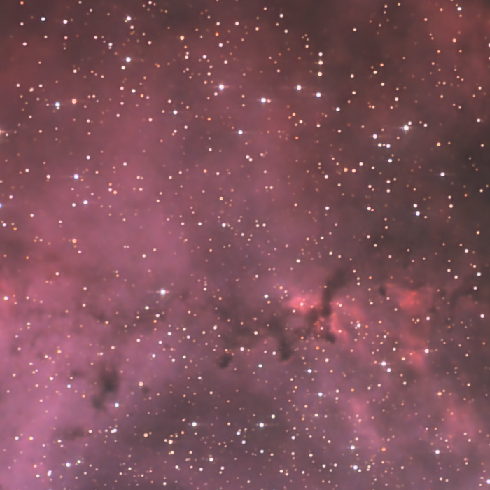 After
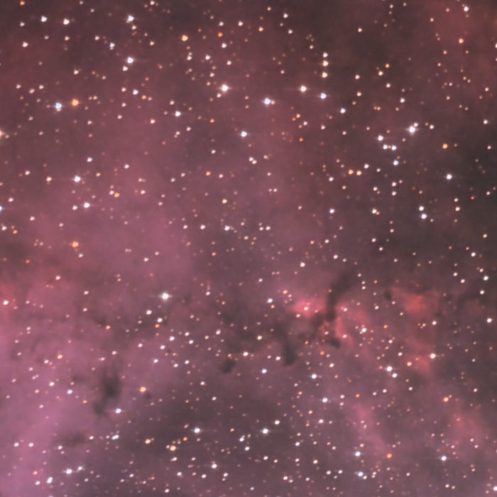 Before
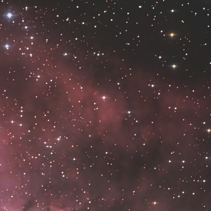 After
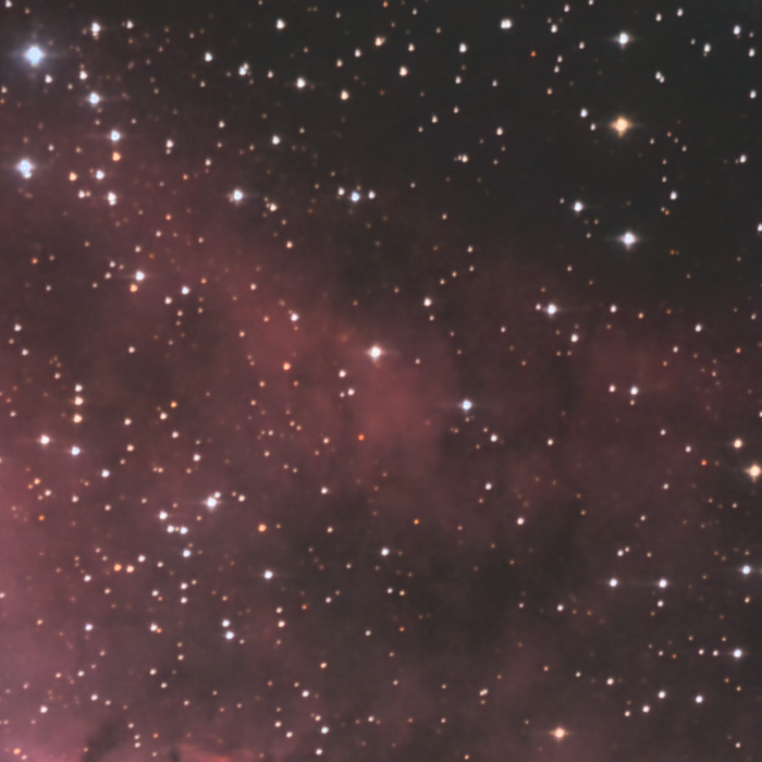 Before
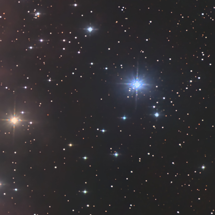 After
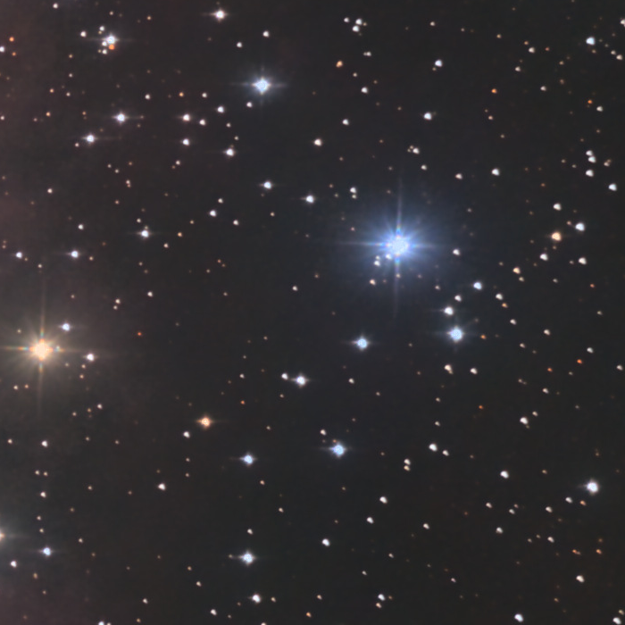 Before
2What goes in, what comes out
The block receives the stack, its two half-stacks, the coverage map of the stack and the map of its saturated pixels. It writes the three images sharpened, a before and after preview, and two measures: the median width of the stars before and after, and the number of zones.
The same operation is applied to the stack and to each half-stack, with the same star shapes, so that a Denoise placed after it still reads two images processed alike, whose difference measures the noise. Pixels without data stay as they were.
3The star shape
The field is cut into zones, with about as many along the short side as keep them square and the number set along the long side (6 by default). In each zone and each colour, FLOAT measures the shape on stars that are:
- not saturated, and not near a saturated pixel or a pixel without data;
- bright: a peak at least 30 times the noise;
- isolated: no neighbour brighter than 3 % of the star within 1.5 times the stamp radius (stamps are 25 × 25 pixels).
Each star is centred to a fraction of a pixel in its own colour, so the small shifts between the colours are not blurred into the shape. The shape of a zone is the median of its stars, normalised to its flux. The faint wings beyond a few pixels from the centre are replaced by the median of the shape around the centre of the star, taken ring by ring, since they are measured with little signal and their noise would weigh like a real halo.
A zone with few stars leans on a smooth model of the field, a quadratic surface fitted to all the zones: a zone’s shape is weighted by its star count against 20 stars of the model, and a zone without stars takes the model. The measured widths, per colour, are written to the log with their range over the zones. Their median, before and after, is the block’s star width measure; it is the width at half height of the shape resampled eight times finer.
If fewer than 10 isolated stars can be found, the star shape cannot be measured: the image is left as it is and the block says so.
4Richardson-Lucy and saturated stars
The method is Richardson-Lucy,[1][2] an iteration that multiplies the estimate by the correction the star shape implies, until the estimate, blurred by that shape, matches the measured image. Each zone is restored with its own shape, and the zones are blended between their centres.[3] The sky is raised to at least 8 noise units above zero during the iterations, since the method needs positive values, and taken back afterwards.
A clipped star would be wrong in a plain Richardson-Lucy. FLOAT follows Whyte, Sivic and Zisserman.[4] At each iteration the estimate is split into its bright pixels and the rest. The measured pixels that the bright ones reach are left out of the update of the rest, which keeps their errors from ringing into the image, and the bright part is updated with a smooth saturation in the forward model. The clipping level of each colour is the high end of the pixels marked saturated in it. After the restoration, the saturated cores themselves are put back as they were photographed.
5Holding back noise and rings
Five mechanisms limit the noise and the rings that deconvolution draws around stars.
- Total variation. A regularisation term holds the noise back.[5] Its strength is the Regularization setting.
- Damped iteration. A pixel already within 3 noise units of the data is no longer pushed (the damping of White[6]).
- Stop. The iteration stops early when the mean relative change of the estimate falls under 0.3 %.
- Local deringing. At each iteration, around the stars, 90 % of a darkening is refused.
- Protection. The result counts in proportion to the signal: not at all under 3 noise units over the sky, in full from 15, so the sky between objects is left alone.
The noise is measured on the difference of the half-stacks, on a sample of at most 2 million pixels drawn with a fixed seed: the same pixels at every run, so the result is the same at every run. The local deringing has no published equation behind it; it is FLOAT’s own rule.
6The neural method (beta)
The second method is a NAFNet network[7] trained against images of the Euclid space telescope. The network ships with the program. This method is in beta.
It works one colour at a time, on the stack and on each half-stack. Each plane is expressed in noise units, passed through the pretrained Denoise network, and then through the deconvolution network, in tiles of 512 pixels with a margin of 48 that fades out over the overlap with the next tile, so that the edges leave no seam. The saturated cores are kept, as in the classic method. The network measures no star shape: it does not read the Zones, Iterations or Regularization settings.
The image goes through Denoise first, and the method also removes the noise. Its star fluxes are less reliable than the classic method’s.
7Settings
| Setting | Value | Range | What it does |
|---|---|---|---|
| Method | Richardson-Lucy | Richardson-Lucy, Neural network (beta) | Richardson-Lucy iterates with the star shape measured across the field. The neural network is in beta and also removes the noise. |
| Iterations | 30 | 1 – 100 | More iterations sharpen more, and raise the noise. Richardson-Lucy only. |
| Regularization | 0.002 | 0 – 0.05 | Holds back noise and ringing. Richardson-Lucy only. |
| Zones (advanced) | 6 | 1 – 16 | Zones along the long side of the image, each with its own measured star shape. Richardson-Lucy only. |
8Limits, and what was tried
- The neural method is in beta. It is not finished. It also removes the noise, and its star fluxes are less reliable than the classic method’s.
- Few stars, no deconvolution. Under 10 isolated, unsaturated stars the image is left as it is. A zone without stars borrows the shape of the model of the field.
- Saturated cores are not restored. The classic method keeps them from ringing; both methods leave them as they were photographed.
- Rings were the difficulty. The damping, the stop, the local deringing and the protection were added against the rings around stars and the noise, with settings frozen on tuning images and judged on 33 others (issue 92). A global deringing step, which gives back part of what went below the measured image, exists in the code and is set to zero.
- Time. On a processor, one colour takes minutes; the neural method also takes minutes per row of tiles.
References
- Richardson, W. H. 1972, Bayesian-Based Iterative Method of Image Restoration, J. Opt. Soc. Am. 62, 55 (Richardson-Lucy). doi:10.1364/JOSA.62.000055
- Lucy, L. B. 1974, An iterative technique for the rectification of observed distributions, AJ 79, 745 (Richardson-Lucy). doi:10.1086/111605
- Nagy, J. G. & O’Leary, D. P. 1998, Restoring Images Degraded by Spatially Variant Blur, SIAM J. Sci. Comput. 19, 1063 (the zones blended between their centres). doi:10.1137/S106482759528507X
- Whyte, O., Sivic, J. & Zisserman, A. 2014, Deblurring Shaken and Partially Saturated Images, International Journal of Computer Vision 110, 185. doi:10.1007/s11263-014-0727-3
- Dey, N. et al. 2006, Richardson-Lucy algorithm with total variation regularization for 3D confocal microscope deconvolution, Microsc. Res. Tech. 69, 260. doi:10.1002/jemt.20294
- White, R. L. 1994, Image restoration using the damped Richardson-Lucy method, Proc. SPIE 2198, 1342, Eqs. 7, 9 and 10. doi:10.1117/12.176819
- Chen, L., Chu, X., Zhang, X. & Sun, J. 2022, Simple Baselines for Image Restoration (NAFNet), ECCV 2022. arXiv:2204.04676